
The ACE801044 is a high-velocity, deterministic hardware accelerator designed for the real-time execution of the QR Givens $4 \times 4$ matrix inversion algorithm. It provides a production-ready "Math-to-Silicon" pipeline that transforms complex mathematics into high-frequency, bit-perfect FPGA logic.
By offloading recursive mathematical kernels from a system’s primary processor, the core enables extreme computational throughput with zero execution jitter. With its >180K operations per second, the ACE801044 may be used in real-time systems avoiding the need to transfer data back and forth between hardware and software.
The core is engineered as a universal mathematical fabric for high-stakes environments. It is specifically optimized for:
The ACE801044 maintains a surprisingly lean resource utilization footprint that enables its implementation on the majority of FPGA models. The core is optimized for the AMD 7 Series FPGA, but ACE can easily port on any customer-selected FPGA (any vendor). While the core is fully functional, ACE internal development procedures provide the possibility for the customer to adapt matrix size, FPGA model, memory map, and core interfaces (e.g., AXI BRAM Controller).
In contrast to software‑based implementations, the ACE801044 delivers architectural guarantees that general‑purpose processors cannot provide. By keeping all data resident inside the FPGA fabric, the core eliminates cache effects, DMA transfers, driver overhead, and any latency associated with moving data between hardware and software—replacing months of low‑level mathematical implementation and numerical‑stability validation with a ready‑to‑use, verified hardware math engine.
xc7k160tfbg484-3
The ACE801044 is a high-performance, deterministic hardware acceleration engine designed to invert $4 \times 4$ matrices by means of QR Givens decomposition. To guarantee minimal, deterministic latency, the engine avoids iterative relaxation methods and utilizes a direct solver architecture split into three highly pipelined, single-precision floating-point (IEEE-754 float32) computational phases:
The engine computes the QR factorization of the input $4 \times 4$ matrix $A \in \mathbb{R}^{4 \times 4}$, decomposing it into an orthogonal matrix $Q$ and an upper triangular matrix $R$, such that:
$$A = Q \cdot R$$
This factorization is achieved through a sequence of 6 distinct Givens rotations designed to systematically annihilate the lower triangular entries of the input matrix. Each rotation operates on a specific plane to clear an off-diagonal element ($a_{ij} \rightarrow 0$) while updating the affected rows. The trigonometric rotation factors ($\cos\theta$ and $\sin\theta$) are evaluated inline using pipelined floating-point square root and division components:
Once the upper triangular matrix $R$ is completely resolved, the engine determines its direct inverse ($R^{-1}$) by executing an inline backward substitution sweep. Because $R$ is upper triangular, the entries of $R^{-1}$ are solved in reverse order starting from the bottom-most scalar entry up to the top row:
The definitive matrix inverse $A^{-1}$ is synthesized by mapping the upper triangular inverse $R^{-1}$ back through the transposed orthogonal rotation matrices. To satisfy matrix transpose laws, the calculation progresses backward through the rotation sequence, propagating the values from the final rotation ($G_6$) down to the first ($G_1$):
$$A^{-1} = R^{-1} Q^T = R^{-1} G_6 G_5 G_4 G_3 G_2 G_1$$
The engine sequentially rotates the columns of the intermediate product matrices utilizing the previously calculated rotation factors $(c_k, s_k)$. Because these operations are entirely unrolled and mapped onto dedicated, deterministic pipelined floating-point primitives, the runtime execution path is strictly bounded and entirely free from timing jitter.
The ACE801044 core utilizes IEEE-754 Single-Precision (32-bit) floating-point arithmetic. The equivalent software implementation is reported below:
function ai = ace801044_inverse(A)
   % ACE801044_INVERSE Self-contained mathematical reference model for the
   % ACE801044 4x4 Givens QR Matrix Inversion Core.

   % Unpack input matrix components into standalone scalar producers
   a00 = A(1,1); a01 = A(1,2); a02 = A(1,3); a03 = A(1,4);
   a10 = A(2,1); a11 = A(2,2); a12 = A(2,3); a13 = A(2,4);
   a20 = A(3,1); a21 = A(3,2); a22 = A(3,3); a23 = A(3,4);
   a30 = A(4,1); a31 = A(4,2); a32 = A(4,3); a33 = A(4,4);

   ONE = 1.0;

   % =========================================================================
   % --- 1. QR DECOMPOSITION (ALL ROTATIONS) ---
   % =========================================================================
   % Rot 1 (A10 -> 0)
   norm1 = sqrt((a00 * a00) + (a10 * a10));
   c1 = a00 / norm1; s1 = (-a10) / norm1;
   r00_v1 = (c1 * a00) - (s1 * a10);
   r01_v1 = (c1 * a01) - (s1 * a11);
   r02_v1 = (c1 * a02) - (s1 * a12);
   r03_v1 = (c1 * a03) - (s1 * a13);
   r11_v1 = (s1 * a01) + (c1 * a11);
   r12_v1 = (s1 * a02) + (c1 * a12);
   r13_v1 = (s1 * a03) + (c1 * a13);

   % Rot 2 (A20 -> 0)
   norm2 = sqrt((r00_v1 * r00_v1) + (a20 * a20));
   c2 = r00_v1 / norm2; s2 = (-a20) / norm2;
   r00_v2 = (c2 * r00_v1) - (s2 * a20);
   r01_v2 = (c2 * r01_v1) - (s2 * a21);
   r02_v2 = (c2 * r02_v1) - (s2 * a22);
   r03_v2 = (c2 * r03_v1) - (s2 * a23);
   r21_v1 = (s2 * r01_v1) + (c2 * a21);
   r22_v1 = (s2 * r02_v1) + (c2 * a22);
   r23_v1 = (s2 * r03_v1) + (c2 * a23);

   % Rot 3 (A30 -> 0)
   norm3 = sqrt((r00_v2 * r00_v2) + (a30 * a30));
   c3 = r00_v2 / norm3; s3 = (-a30) / norm3;
   r00 = (c3 * r00_v2) - (s3 * a30);
   r01 = (c3 * r01_v2) - (s3 * a31);
   r02 = (c3 * r02_v2) - (s3 * a32);
   r03 = (c3 * r03_v2) - (s3 * a33);
   r31_v1 = (s3 * r01_v2) + (c3 * a31);
   r32_v1 = (s3 * r02_v2) + (c3 * a32);
   r33_v1 = (s3 * r03_v2) + (c3 * a33);

   % Rot 4 (r21_v1 -> 0)
   norm4 = sqrt((r11_v1 * r11_v1) + (r21_v1 * r21_v1));
   c4 = r11_v1 / norm4; s4 = (-r21_v1) / norm4;
   r11_v2 = (c4 * r11_v1) - (s4 * r21_v1);
   r12_v2 = (c4 * r12_v1) - (s4 * r22_v1);
   r13_v2 = (c4 * r13_v1) - (s4 * r23_v1);
   r22_v2 = (s4 * r12_v1) + (c4 * r22_v1);
   r23_v2 = (s4 * r13_v1) + (c4 * r23_v1);

   % Rot 5 (r31_v1 -> 0)
   norm5 = sqrt((r11_v2 * r11_v2) + (r31_v1 * r31_v1));
   c5 = r11_v2 / norm5; s5 = (-r31_v1) / norm5;
   r11 = (c5 * r11_v2) - (s5 * r31_v1);
   r12 = (c5 * r12_v2) - (s5 * r32_v1);
   r13 = (c5 * r13_v2) - (s5 * r33_v1);
   r32_v2 = (s5 * r12_v2) + (c5 * r32_v1);
   r33_v2 = (s5 * r13_v2) + (c5 * r33_v1);

   % Rot 6 (r32_v2 -> 0)
   norm6 = sqrt((r22_v2 * r22_v2) + (r32_v2 * r32_v2));
   c6 = r22_v2 / norm6; s6 = (-r32_v2) / norm6;
   r22 = (c6 * r22_v2) - (s6 * r32_v2);
   r23 = (c6 * r23_v2) - (s6 * r33_v2);
   r33 = (s6 * r23_v2) + (c6 * r33_v2);

   % =========================================================================
   % --- 2. BACK-SUBSTITUTION (R_inv) ---
   % =========================================================================
   x33 = ONE / r33; x22 = ONE / r22; x11 = ONE / r11; x00 = ONE / r00;
   x23 = (-r23) * x33 * x22;
   x12 = (-r12) * x22 * x11;
   x13 = (((-r12) * x23) + ((-r13) * x33)) * x11;
   x01 = (-r01) * x11 * x00;
   x02 = (((-r01) * x12) + ((-r02) * x22)) * x00;
   x03 = (((-r01) * x13) + ((-r02) * x23) + ((-r03) * x33)) * x00;

   % =========================================================================
   % --- 3. FINAL INVERSE (A_inv) via Retrograde Right-Multiplication ---
   % =========================================================================
   % Step 3.1: Apply Q6 (Columns 2 & 3)
   g02_v1 = (c6 * x02) + (s6 * x03); g03_v1 = -(s6 * x02) + (c6 * x03);
   g12_v1 = (c6 * x12) + (s6 * x13); g13_v1 = -(s6 * x12) + (c6 * x13);
   g22_v1 = (c6 * x22) + (s6 * x23); g23_v1 = -(s6 * x22) + (c6 * x23);
   g32_v1 = s6 * x33;                g33_v1 = c6 * x33;

   % Step 3.2: Apply Q5 (Columns 1 & 3)
   g01_v1 = (c5 * x01) + (s5 * g03_v1); g03_v2 = -(s5 * x01) + (c5 * g03_v1);
   g11_v1 = (c5 * x11) + (s5 * g13_v1); g13_v2 = -(s5 * x11) + (c5 * g13_v1);
   g21_v1 = s5 * g23_v1;                g23_v2 = c5 * g23_v1;
   g31_v1 = s5 * g33_v1;                g33_v2 = c5 * g33_v1;

   % Step 3.3: Apply Q4 (Columns 1 & 2)
   g01_v2 = (c4 * g01_v1) + (s4 * g02_v1); g02_v2 = -(s4 * g01_v1) + (c4 * g02_v1);
   g11_v2 = (c4 * g11_v1) + (s4 * g12_v1); g12_v2 = -(s4 * g11_v1) + (c4 * g12_v1);
   g21_v2 = (c4 * g21_v1) + (s4 * g22_v1); g22_v2 = -(s4 * g21_v1) + (c4 * g22_v1);
   g31_v2 = (c4 * g31_v1) + (s4 * g32_v1); g32_v2 = -(s4 * g31_v1) + (c4 * g32_v1);

   % Step 3.4: Apply Q3 (Columns 0 & 3)
   g00_v1 = (c3 * x00) + (s3 * g03_v2); ai03 = -(s3 * x00) + (c3 * g03_v2);
   g10_v1 = s3 * g13_v2;                ai13 = c3 * g13_v2;
   g20_v1 = s3 * g23_v2;                ai23 = c3 * g23_v2;
   g30_v1 = s3 * g33_v2;                ai33 = c3 * g33_v2;

   % Step 3.5: Apply Q2 (Columns 0 & 2)
   g00_v2 = (c2 * g00_v1) + (s2 * g02_v2); ai02 = -(s2 * g00_v1) + (c2 * g02_v2);
   g10_v2 = (c2 * g10_v1) + (s2 * g12_v2); ai12 = -(s2 * g10_v1) + (c2 * g12_v2);
   g20_v2 = (c2 * g20_v1) + (s2 * g22_v2); ai22 = -(s2 * g20_v1) + (c2 * g22_v2);
   g30_v2 = (c2 * g30_v1) + (s2 * g32_v2); ai32 = -(s2 * g30_v1) + (c2 * g32_v2);

   % Step 3.6: Apply Q1 (Columns 0 & 1)
   ai00 = (c1 * g00_v2) + (s1 * g01_v2); ai01 = -(s1 * g00_v2) + (c1 * g01_v2);
   ai10 = (c1 * g10_v2) + (s1 * g11_v2); ai11 = -(s1 * g10_v2) + (c1 * g11_v2);
   ai20 = (c1 * g20_v2) + (s1 * g21_v2); ai21 = -(s1 * g20_v2) + (c1 * g21_v2);
   ai30 = (c1 * g30_v2) + (s1 * g31_v2); ai31 = -(s1 * g30_v2) + (c1 * g31_v2);

   ai = [ ai00, ai01, ai02, ai03;
          ai10, ai11, ai12, ai13;
          ai20, ai21, ai22, ai23;
          ai30, ai31, ai32, ai33 ];
end
The data below are representative of the AMD 7 series architecture. The percentages are relative to the budget-friendly xc7k160tfbg484-3:
The core runs on two different clocks:
CLK_FAST with a maximum frequency of 250 MHzCLK_SLOW that shall run at 50 MHz (phase aligned with CLK_FAST)
CLK_SLOW is used for the ACE801044 initialization, while CLK_FAST is used for all runtime operations. In the verification project, timing was closed with a robust 0.755 ns timing margin and with 0 timing violations.
The QR Givens $4 \times 4$ Inverter core is packaged as an AMD IP core. Figure 1 illustrates the verification configuration.
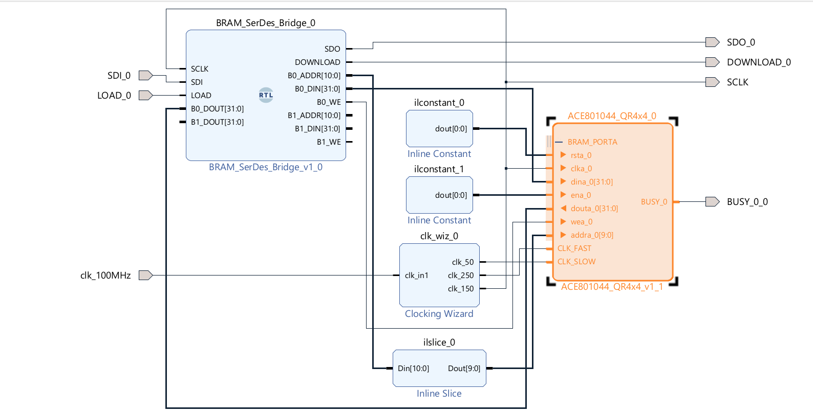
The core is fully controlled through read/write operations on a BRAM (optionally accessible via an AXI BRAM_CONTROLLER). The instantiated BRAM is 1 True Dual Port with port A available to the user and port B managed by the internal Math Engine. The BRAM has a width of 32 bits and a depth of 1024 locations. The core uses the first 128 locations (0–127), with the remaining ones completely available for the user via port A.
| ID | ADDRESS | VARIABLE | DIR | FORMAT | Note |
|---|---|---|---|---|---|
| BRAM_0 | 0 | START_CMD | IN-OUT | BINARY | Set to 0x1 by the user to start the computation. Set to 0x0 by the math engine at the end of computation. |
| BRAM_0 | 1 | DNA1 | OUT | BINARY | FPGA DNA (MSB) populated after initialization. |
| BRAM_0 | 2 | DNA2 | OUT | BINARY | FPGA DNA (LSB) populated after initialization. |
| BRAM_0 | 3 | USER_KEY1 | IN | BINARY | LICENSE_KEY (MSB) input required for validation. |
| BRAM_0 | 4 | USER_KEY2 | IN | BINARY | LICENSE_KEY (LSB) input required for validation. |
| BRAM_0 | 5 .. 20 | a00 .. a33 | IN | FLOAT32 | Input matrix $A$ elements in row-major order ($a_{00}, a_{01}, \dots, a_{33}$). |
| BRAM_0 | 21 .. 36 | ai00 .. ai33 | OUT | FLOAT32 | Inverted matrix $A^{-1}$ result elements in row-major order ($ai_{00}, ai_{01}, \dots, ai_{33}$). |
| BRAM_0 | 37 .. 127 | Intermediate Computations | N/A | RESERVED | DON'T TOUCH — Internal engine scratchpad registers. |
In addition to the BRAM interface, the core exposes:
CLK_SLOW is used for the initialization and for access to the DNA reader primitive ($50\text{ MHz}$)CLK_FAST is used to drive the internal computation engine (Max Frequency: $250\text{ MHz}$)BUSY pin that, when set to high, signals when the core is executing the initialization or its main function.
The core, at power-up, performs an initialization sequence that lasts (with CLK_SLOW @ $50\text{ MHz}$) less than $5,000\text{ ns}$, populating the BRAM with the DNA of the FPGA. Once initialized, the user loads the BRAM inputs and sets START_CMD to 0x1.
The results are written in BRAM, in accordance with the memory map, after exactly 1,384 clock cycles ($5.536\ \mu\text{s}$ @ $250\text{ MHz}$). The end of execution is communicated by the core by setting START_CMD to 0x0 (in BRAM) and via the BUSY pin (BUSY=0 indicates IDLE state, ready for the next execution).
Note: if the USER_KEY is not correct, the core terminates in the specified timeframe, but produces unpredictable results.
To validate the numerical integrity and dynamic range stability of the ACE801044 computing fabric, the hardware engine was subjected to a rigorous, 10-stage hardware-in-the-loop simulation test sweep. The verification manifest intentionally sweeps the input matrix ($A$) across diverse operational ranges, forcing the internal single-precision floating-point (float32) pipelines to calculate direct matrix inversions under varying conditioning states.
As compiled in the hardware bit-fidelity verification report below, the core achieved 100% numerical equivalence with zero precision breaches across all evaluated operating envelopes. Maximum observed epsilon drift was bounded in the sub-fractional nano-signal space, peaking at $3.54 \times 10^{-8}$ under peak stress loading (Stage 6), while nominal tracking bounds routinely converged well below $1.19 \times 10^{-8}$ drift (Stage 2), demonstrating true IEEE-754 bit-perfect math propagation.
=========================================================
 ACE801044 BIT-FIDELITY VERIFICATION REPORT
=========================================================
---------------------------------------------------------
 EVALUATION RESULTS FOR: STAGE_1
---------------------------------------------------------
 VERDICT: [PASS]
 Maximum Observed Epsilon Drift: 2.411946e-08

 Original Input Matrix (A):
    5.5377    0.3188    3.5784    0.7254
    1.8339   -6.3077    2.7694   -0.0631
   -2.2588   -0.4336   -6.3499    0.7147
    0.8622    0.3426    3.0349   -5.2050

 Hardware Computed Matrix Inverse (A^-1):
    0.2365    0.0039    0.1613    0.0551
    0.0305   -0.1536   -0.0502   -0.0008
   -0.0873    0.0086   -0.2235   -0.0430
   -0.0097   -0.0044   -0.1069   -0.2081

 Golden Model Analytical Matrix Inverse:
    0.2365    0.0039    0.1613    0.0551
    0.0305   -0.1536   -0.0502   -0.0008
   -0.0873    0.0086   -0.2235   -0.0430
   -0.0097   -0.0044   -0.1069   -0.2081

---------------------------------------------------------
 EVALUATION RESULTS FOR: STAGE_2
---------------------------------------------------------
 VERDICT: [PASS]
 Maximum Observed Epsilon Drift: 1.189276e-08

 Original Input Matrix (A):
   -5.1241    0.6715    0.4889    0.2939
    1.4897   -6.2075    1.0347   -0.7873
    1.4090    0.7172    5.7269    0.8884
    1.4172    1.6302   -0.3034   -6.1471

 Hardware Computed Matrix Inverse (A^-1):
   -0.1965   -0.0200    0.0202   -0.0039
   -0.0299   -0.1546    0.0317    0.0230
    0.0608    0.0316    0.1649    0.0227
   -0.0562   -0.0472    0.0049   -0.1586

 Golden Model Analytical Matrix Inverse:
   -0.1965   -0.0200    0.0202   -0.0039
   -0.0299   -0.1546    0.0317    0.0230
    0.0608    0.0316    0.1649    0.0227
   -0.0562   -0.0472    0.0049   -0.1586

---------------------------------------------------------
 EVALUATION RESULTS FOR: STAGE_6 (PEAK STRESS)
---------------------------------------------------------
 VERDICT: [PASS]
 Maximum Observed Epsilon Drift: 3.541629e-08

 Original Input Matrix (A):
    6.4193   -0.8045    0.2157    0.7223
    0.2916    5.6966   -1.1658    2.5855
    0.1978    0.8351   -6.1480   -0.6669
    1.5877   -0.2437    0.1049    5.1873

 Hardware Computed Matrix Inverse (A^-1):
    0.1630    0.0214    0.0011   -0.0332
    0.0167    0.1789   -0.0350   -0.0960
    0.0129    0.0248   -0.1675   -0.0357
   -0.0494    0.0013    0.0014    0.1992

 Golden Model Analytical Matrix Inverse:
    0.1630    0.0214    0.0011   -0.0332
    0.0167    0.1789   -0.0350   -0.0960
    0.0129    0.0248   -0.1675   -0.0357
   -0.0494    0.0013    0.0014    0.1992

---------------------------------------------------------
 EVALUATION RESULTS FOR: STAGE_10
---------------------------------------------------------
 VERDICT: [PASS]
 Maximum Observed Epsilon Drift: 2.309516e-08

 Original Input Matrix (A):
   -5.8314   -2.0026   -0.0348   -0.7145
   -0.9792    5.9642   -0.7982    1.3514
   -1.1564    0.5201    6.0187   -0.2248
   -0.5336   -0.0200   -0.1332   -5.5890

 Hardware Computed Matrix Inverse (A^-1):
   -0.1617   -0.0536   -0.0079    0.0080
   -0.0339    0.1546    0.0212    0.0409
   -0.0275   -0.0235    0.1627   -0.0087
    0.0162    0.0051   -0.0032   -0.1796

 Golden Model Analytical Matrix Inverse:
   -0.1617   -0.0536   -0.0079    0.0080
   -0.0339    0.1546    0.0212    0.0409
   -0.0275   -0.0235    0.1627   -0.0087
    0.0162    0.0051   -0.0032   -0.1796

=========================================================
 FINAL REPORT: SUCCESS (All 10 stages match within verification limit)
=========================================================ACE801044 is delivered as a pre‑packaged Vivado IP core, ready for integration through the AMD/Xilinx IP Catalog. Each licensed core includes:
USER_KEY file for license activation
ACE provides a USER_KEY value (64 bits) for FPGA Serial Number (DNA for AMD/Xilinx). The keys are delivered in a simple CSV file:
DNA_HEX,AUTHORIZATION_KEY
0011223344556677,C303E222F7D44C5B
ABCDE1234567890F,A2A3A3114194ED74
5566778899AABBCC,94C023F594AA6F63
DEADBEEF12345678,F40237F85DFB6F2A
00123456789ABCDE,E8ACBBDBFCF3ACB7
...............,.................BRAM_PORTA interface (addresses 1 and 2).USER_KEY corresponding to the FPGA SN in the ACE provided USER_KEY file.USER_KEY via the BRAM_PORTA interface (addresses 3 and 4).
The keys are generated on customer order. In simulation, a demo DNA is used and the corresponding USER_KEY is provided in the file for a seamless experience.
Pricing is provided directly by ACE based on deployment volume, license type, optional customization requirements, and target FPGA family.
Data Privacy note: By contacting us via email, you agree that we will use your provided contact details and mathematical specifications solely to evaluate project feasibility during our early-access phase. We do not sell or share your personal information with third parties. We may use standard web analytics tools to monitor basic, aggregated website traffic to improve our site performance.